Define Transition Matrix for Markov Model

Define a matrix of transition probabilities. Probability can depend on parameters defined with define_parameters(), and can thus be time-dependent.

Usage

define_transition(..., state_names)

define_transition_(.dots, state_names)

# S3 method for class 'uneval_matrix'
modify(.OBJECT, ...)

# S3 method for class 'uneval_matrix'
plot(x, relsize = 0.75, shadow.size = 0, latex = TRUE, ...)

Arguments

...

Name-value pairs of expressions defining matrix cells. Can refer to parameters defined with define_parameters(). For plot, additional arguments passed to diagram::plotmat().

state_names

character vector, optional. State names.

.dots

Used to work around non-standard evaluation.

.OBJECT

An object of class uneval_matrix.

x

An uneval_matrix to plot.

relsize

Argument passed to diagram::plotmat().

shadow.size

Argument passed to diagram::plotmat().

latex

Argument passed to diagram::plotmat().

Value

An object of class uneval_matrix (actually a named list of quosures expressions).

Details

Matric cells are listed by row.

Parameters names are searched first in a parameter object defined with define_parameters() and linked with the matrix through define_strategy(); then in the environment where the matrix was defined.

The complementary probability of all other row probabilities can be conveniently referred to as C.

The matrix code can be re-indented for readability with reindent_transition().

Only matrix size is checked during this step (the matrix must be square). Other conditions (such as row sums being equal to 1) are tested later, during model evaluation.

For the modify function, existing matrix cells are replaced with the new expression. Cells are referenced by name. Cell naming follows the cell_x_y convention, with x being the row number and y the column number.

Examples

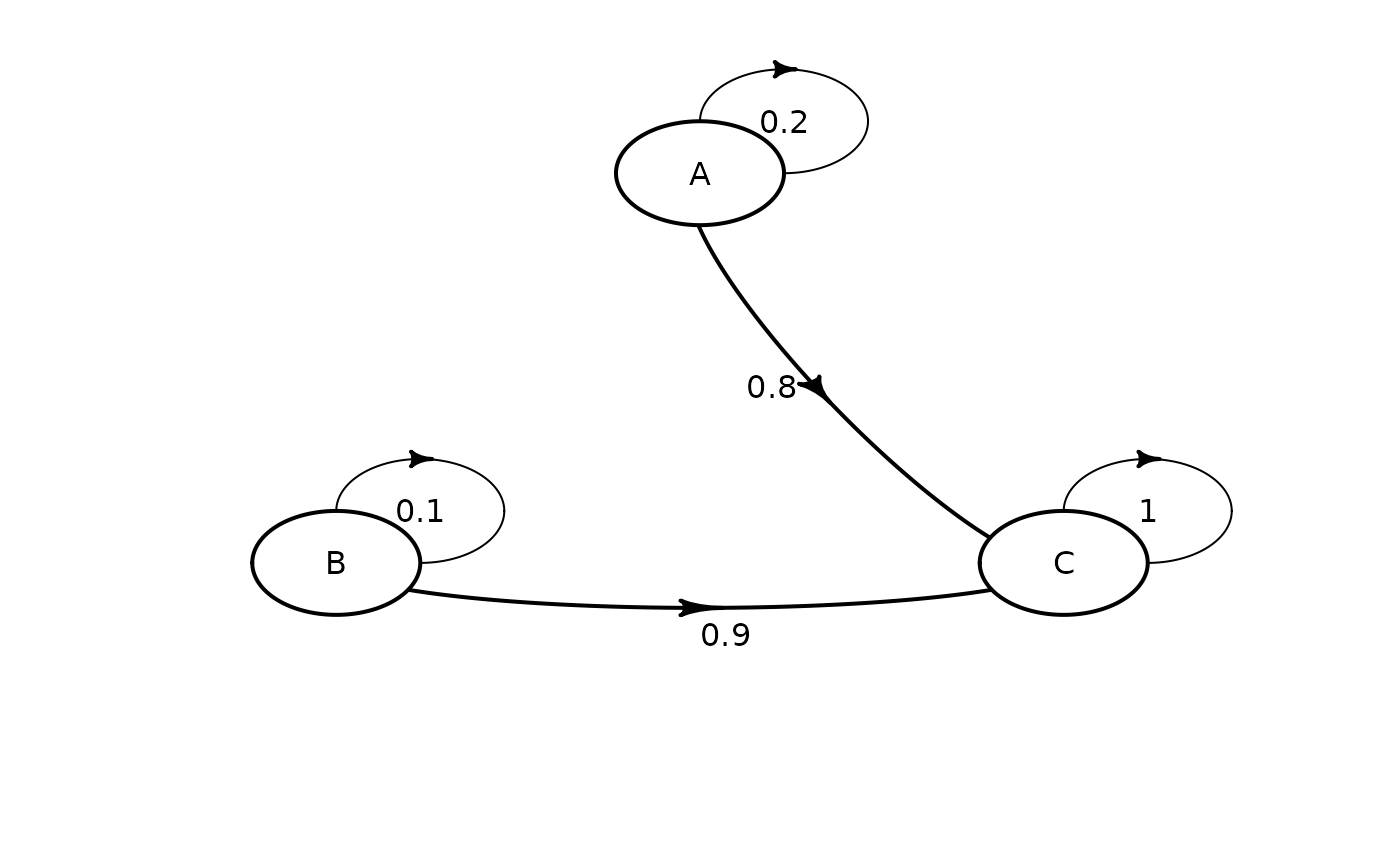
# simple 3x3 transition matrix

mat_1 <- define_transition(
  .2, 0, .8,
  0, .1, .9,
  0, 0, 1
)
#> No named state -> generating names.
mat_1
#> A transition matrix, 3 states.
#> 
#>   A   B   C  
#> A 0.2     0.8
#> B     0.1 0.9
#> C         1  

plot(mat_1)
#> Loading required namespace: diagram


# referencing parameters
# rr must be present in a parameter object
# that must later be linked with define_strategy

mat_2 <- define_transition(
  .5 - rr, rr,
  .4, .6
)
#> No named state -> generating names.
mat_2
#> A transition matrix, 2 states.
#> 
#>   A        B  
#> A 0.5 - rr rr 
#> B 0.4      0.6

reindent_transition(mat_2)
#> Loading required namespace: stringr
#> state_names = c(
#> "A"     , "B")
#> 0.5 - rr, rr ,
#> 0.4     , 0.6

# can also use C

define_transition(
  C, rr,
  .4, .6
)
#> No named state -> generating names.
#> A transition matrix, 2 states.
#> 
#>   A   B  
#> A C   rr 
#> B 0.4 0.6

# updating cells from mat_1

modify(
  mat_1,
  cell_2_1 = .2,
  cell_2_3 = .7
)
#> A transition matrix, 3 states.
#> 
#>   A   B   C  
#> A 0.2     0.8
#> B 0.2 0.1 0.7
#> C         1  

# only matrix size is check, it is thus possible
# to define an incorrect matrix

# this matrix will generate an error later,
# during model evaluation

define_transition(
  .5, 3,
  -1, 2
)
#> No named state -> generating names.
#> A transition matrix, 2 states.
#> 
#>   A   B
#> A 0.5 3
#> B -1  2