Tabular Input

In most of the heemod vignettes models are defined through R code. But models with large numbers of states and transition probabilities might be unwieldy to input at the keyboard, and could be conveniently specified by file inputs.

This vignette demonstrates how to make and use files to input models to heemod. The files can then be used to run a suite of analyses (including deterministic and probabilistic sensitivity analyses, acceptability curve calculation, etc.) and optionally save results to a folder.

Introduction

The inputs for state definition, transition matrices, model options, etc. (referenced as tabular inputs) must be provided via csv, xls or xlsx files.¹ Columns starting by .comment are ignored, as well as blank rows.

These inputs must be provided in separate files. The path to these files is specified in a reference file, that acts as an ‘umbrella’ file atop of the other inputs. The reference file default name is REFERENCE.csv.

Warning for users of the xls format:
The xls files are read with the readxl package. As of version 0.1.1 if a column contains strings and numeric values the numeric values are rounded to 6 decimal places. We therefore recommend to use solely the csv or xlsx format.

Reference file

This file contains two mandatory columns data and file, as well as optional columns with comments, which will be ignored. The data column must contain the following keywords:

state: file containing model states.
tm: file containing transition probabilities.
parameters: file containing model parameters.

Optionally, the following rows can be provided:

options: file specifying model options.
demographics: file describing of the population to run the models on.
data: a directory containing additional tables to be loaded; these can be .csv, .xls or .xlsx.
output: a directory to save the output graphics.
source: a directory in which R source files used in the analysis can be placed, and will be sourced when the model is run. The global environment is not modified.

data	file
state	THR_states.csv
tm	THR_transition_probs.csv
parameters	THR_parameters.csv
demographics	THR_demographic_table.csv
data	input_dataframes
output	output
options	THR_options.csv

All the files and directories must be in the reference file directory. Files or directories located elsewhere must be given by absolute path and marked by a TRUE value in an optional absolute_path column.

States file

A state file contains 2 mandatory columns: .model and .state, corresponding to strategy and state names respectively. The other columns correspond to the state values.

Discounting rates can be specified in .discount.* columns, where * stands for the name of the value to discount. Values are always discounted at the same rate in all states.²

Values specified for only one strategy will be carried over to others. Only values that differ from one strategy to another must be specified separately for each strategy.

.model	.state	cost	qaly	.discount.qaly
standard	PrimaryTHR	0	0.00	0.015
standard	SuccessfulPrimary	0	0.85
standard	RevisionTHR	5294	0.30
standard	SuccessfulRevision	0	0.75
standard	Death	0	0.00
new	PrimaryTHR	0	0.00	0.015

State values that do not change between models need only be specified once (such as all states except PrimaryTHR in the new model) and will automatically be repeated between models.

Transition probabilities

A transition probabilities file contains 4 columns:

.model: strategy name.
from: initial state.
to: end state.
prob: transition probability from initial state to end state.

.model	from	to	prob
standard	PrimaryTHR	SuccessfulPrimary	C
standard	PrimaryTHR	Death	0.02
standard	SuccessfulPrimary	SuccessfulPrimary	C
standard	SuccessfulPrimary	RevisionTHR	pHRFailStandard
standard	SuccessfulPrimary	Death	mr
standard	RevisionTHR	SuccessfulRevision	C
standard	RevisionTHR	Death	0.02+mr
standard	SuccessfulRevision	SuccessfulRevision	C
standard	SuccessfulRevision	RevisionTHR	0.04
standard	SuccessfulRevision	Death	mr
standard	Death	Death	1
new	SuccessfulPrimary	RevisionTHR	pHRFailNew

A probability can be defined by any expression: a number, C, a different parameter name (specified in the parameter file), or a function call.

As with the state file above probabilities specified for only one strategy will be carried over to others. Only probabilities that differ from one strategy to another must be specified separately for each strategy. Unspecified transition probabilities are assumed to be 0.

Parameters

A parameter file contains 2 mandatory columns: the parameter names parameter and the values value.

Optional columns can be added to perform deterministic or probabilistic sensitivity analysis (DSA and PSA). low and high columns specify the lower and upper bounds of parameter values for DSA, while psa contains the parameter distribution for PSA.

parameter	value	low	high	psa
lngamma	0.3740968	0.2791966	0.468997	normal(0.27, 0.001)
gamma	exp(lngamma)
constant	-5.490935	-5.906719	-5.075151
agecoef	-0.0367022	-0.0471246	-0.0262798	normal(-0.04, 0.001)
malecoef	0.768536	0.550404	0.986668
np1	-1.344474	-2.109637	-0.579311
rr	exp(np1)	0.121282	0.5602843	binomial(0.12, 500)
age_init	60
age	age_init + model_time
sex	0
sex_str	ifelse(sex==1, “Males”, “Females”)
mr	look_up(mr_table, age = age, sex = sex_str, bin = TRUE, value = “value”)
lambdaStandard	exp(constant + agecoef * age_init + malecoef * sex)
lambdaNew	exp(constant + agecoef * age_init + malecoef * sex) * rr
pHRFailStandard	1 - exp(lambdaStandard * ((model_time-1)^gamma - model_time^gamma))
pHRFailNew	1 - exp(lambdaNew * ((model_time-1)^gamma - model_time^gamma))

A parameter can be specified as any expression: as a number, through a previously defined parameter, with a mathematical formula or a function call.

The look_up() function can be used to look up parameter values in external reference tables (see section User-defined data), if a data argument is given in the reference file (as for the mr parameter in the above example).

User-defined data

Sometimes external data is required for an analysis (e.g. age-specific mortality rates). A data row in the reference file specifies a subdirectory containing data frames to be loaded (saved as csv, xls, or xlsx files). Multiple files can be placed here, and each filename (without the extension) is used as the dataframe name.³

Model options

Models specified by tabular input will run with defaults options. The following options can be specified in a non-mandatory options file:

cost, effect: values to be used as cost and effect.
init comma separated starting values.
method: counting method.
base: name of base model.
cycles: run the model for how many cycles?
n: number of resample for PSA.
num_core: number of cluster cores.

option	value
cost	cost
effect	qaly
method	beginning
cycles	50
n	10
init	1000, 0, 0, 0, 0

Run the analysis

The entire set of analysis specified in the tabular files can be run by the function run_model_from_tabular().

result <- run_model_tabular(
  location = system.file("tabular/thr", package = "heemod")
)

## Running DSA on strategy 'standard'...

## Running DSA on strategy 'new'...

## Resampling strategy 'standard'...
## Resampling strategy 'standard'...

## Resampling strategy 'new'...
## Resampling strategy 'new'...

## Updating strategy 'standard'...

## Updating strategy 'new'...

The results can then be interpreted as usual.

result$model_runs

## 2 strategies run for 50 cycles.
## 
## Initial state counts:
## 
## PrimaryTHR = 1000
## SuccessfulPrimary = 0
## RevisionTHR = 0
## SuccessfulRevision = 0
## Death = 0
## 
## Counting method: 'beginning'.
## 
## Values:
## 
##               cost     qaly
## standard 304266.73 14641.51
## new       80960.18 14685.77
## 
## Efficiency frontier:
## 
## new
## 
## Differences:
## 
##     Cost Diff. Effect Diff.      ICER     Ref.
## new  -223.3065   0.04426563 -5044.693 standard

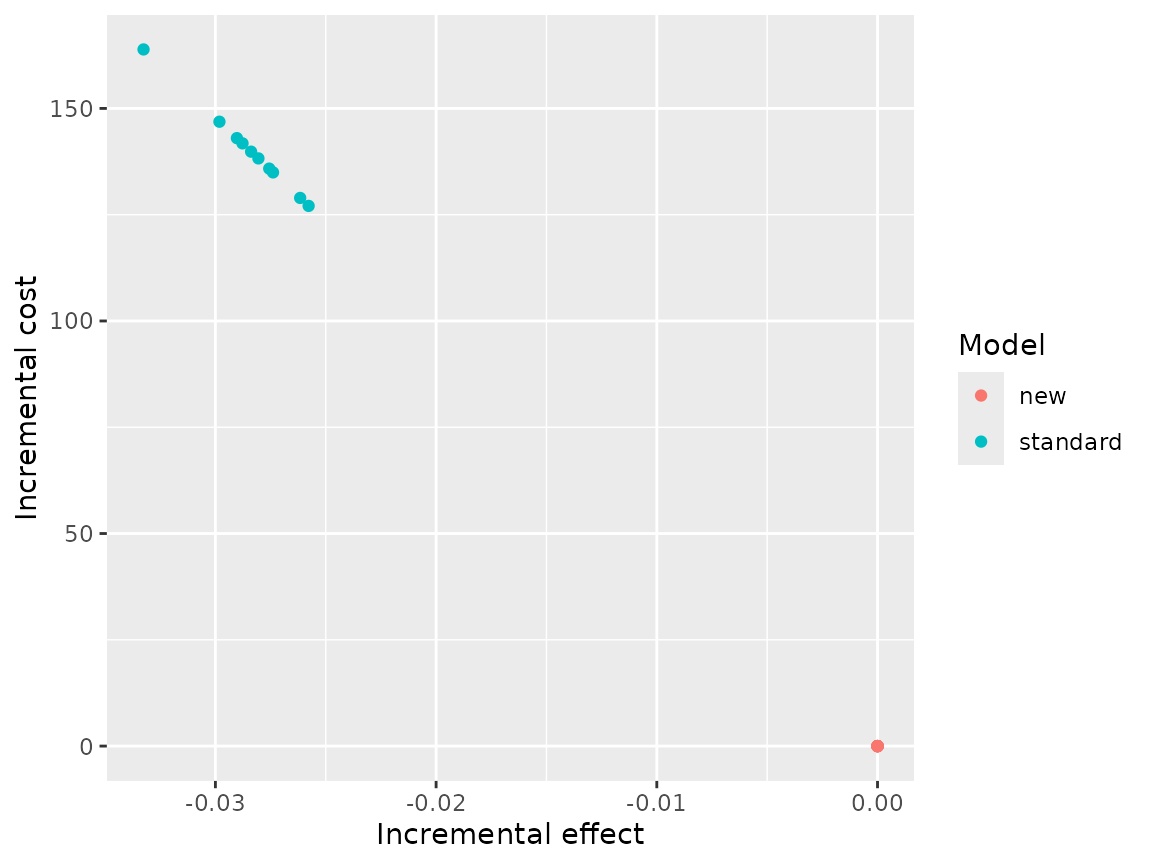
plot(result$psa,
     type = "ce")

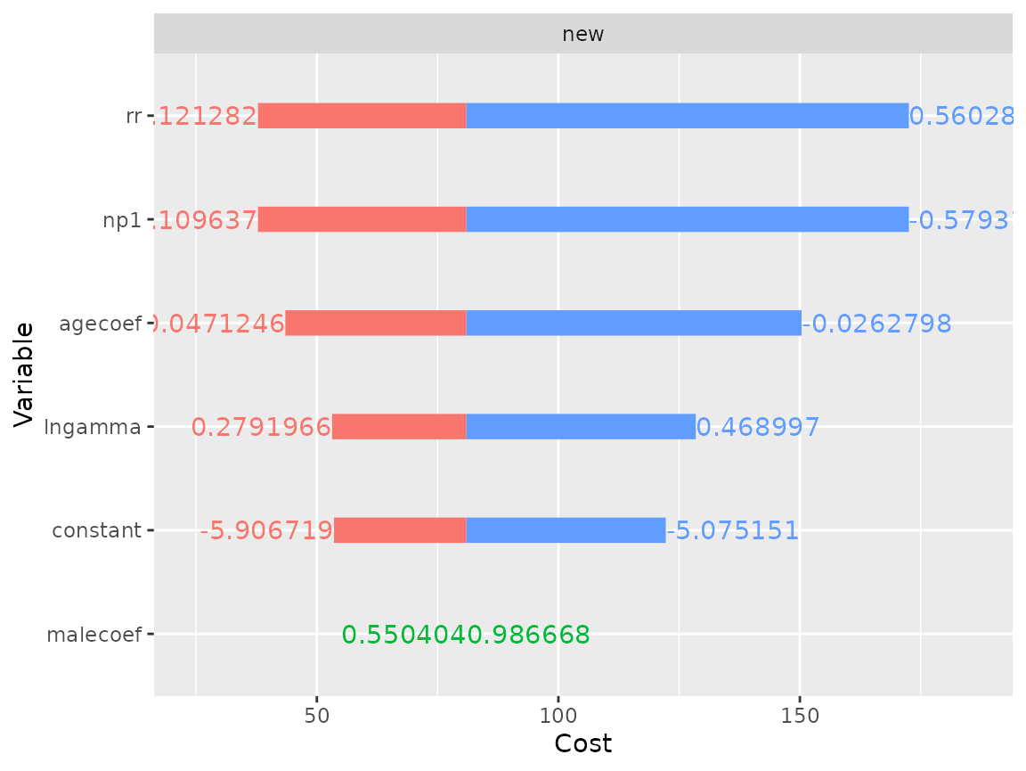
plot(result$dsa,
     result = "cost",
     strategy = "new")

result$demographics

## An analysis re-run on 8 parameter sets.
## 
## * Weights distribution:
## 
##    Min. 1st Qu.  Median    Mean 3rd Qu.    Max. 
## 0.00219 0.01194 0.01482 0.01489 0.01994 0.02264 
## 
## Total weight: 0.1191407
## 
## * Values distribution:
## 
##                                  Min.       1st Qu.        Median          Mean
## standard - Cost          3.892620e+01  4.392518e+01   993.2017848   708.5801137
## standard - Effect        4.098947e+00  4.403150e+00    13.1467098    10.0487221
## standard - Cost Diff.               -             -             -             -
## standard - Effect Diff.             -             -             -             -
## standard - Icer                     -             -             -             -
## new - Cost               1.022389e+01  1.154223e+01   279.3495600   200.4971884
## new - Effect             4.103704e+00  4.408382e+00    13.2912790    10.1504406
## new - Cost Diff.        -9.174158e+02 -8.167007e+02  -713.8522248  -508.0829253
## new - Effect Diff.       4.587073e-03  5.172165e-03     0.1418194     0.1017185
## new - Icer              -6.263848e+03 -6.256979e+03 -5032.9834879 -5471.8546606
##                               3rd Qu.          Max.
## standard - Cost          1139.7822107  1284.1587856
## standard - Effect          13.8274561    14.4422790
## standard - Cost Diff.               -             -
## standard - Effect Diff.             -             -
## standard - Icer                     -             -
## new - Cost                323.0815351   366.7429773
## new - Effect               13.9929427    14.6290526
## new - Cost Diff.          -32.3829481   -28.7023186
## new - Effect Diff.          0.1643751     0.1867736
## new - Icer              -4968.9381888 -4911.9130861
## 
## * Combined result:
## 
## 2 strategies run for 50 cycles.
## 
## Initial state counts:
## 
## PrimaryTHR = 1000
## SuccessfulPrimary = 0
## RevisionTHR = 0
## SuccessfulRevision = 0
## Death = 0
## 
## Counting method: 'beginning'.
## 
## Values:
## 
##              cost     qaly
## standard 708580.1 10048.72
## new      200497.2 10150.44
## 
## Efficiency frontier:
## 
## new
## 
## Differences:
## 
##     Cost Diff. Effect Diff.      ICER     Ref.
## new  -508.0829    0.1017185 -4994.989 standard

2024-09-11